Infinite Script

What’s a decision tree?

A decision tree is a flowchart-like structure in which each internal node represents a "test" on an attribute (e.g. whether a coin flip comes up heads or tails), each branch represents the outcome of the test and each leaf node represents a class label (decision taken after computing all attributes). The paths from root to leaf represent classification rules.

Overview

A decision tree is a flowchart-like structure in which each internal node represents a "test" on an attribute (e.g. whether a coin flip comes up heads or tails), each branch represents the outcome of the test and each leaf node represents a class label (decision taken after computing all attributes). The paths from root to leaf represent classification rules.

A decision tree consists of 3 types of nodes:

• Decision nodes - commonly represented by squares
• Chance nodes - represented by circles
• End nodes - represented by triangles

An example of a decision tree goes below:

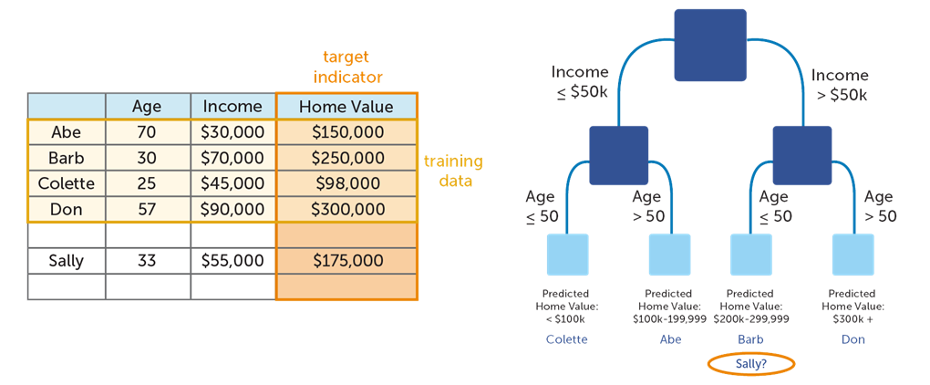
We get a decision tree using training data: Abe, Barb, Colette, and Don. And we can get Home value of Sally using this decision tree.

Metrics

Information Gain

What’s entropy?

Entropy (very common in Information Theory) characterizes the impurity of an arbitrary collection of examples.

We can calculate the entropy as follows:

$entropy(p)=\sum\limits_{i=1}^n{P_i}\log{P_i}$

For example, for the set $R = \{a, a, a, b, b, b, b, b\}$

$entropy(R)=-\frac{3}{8}\log\frac{3}{8}-\frac{5}{8}\log\frac{5}{8}$

What’s information entropy?

In general terms, the expected information gain is the change in information entropy H from a prior state to a state that takes some information as given:

$IG(D,A)=\Delta{Entropy}=Entropy(D)-Entropy(D|A)$

Take the image below as an example:

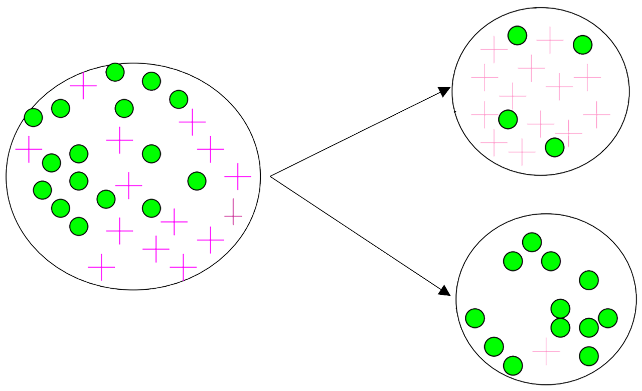
The entropy before splitting: $Entropy(D)=-\frac{14}{30}\log\frac{14}{30}-\frac{16}{30}\log\frac{16}{30}\approx{0.996}$

The entropy after splitting: $Entropy(D|A)=-\frac{17}{30}(\frac{13}{17}\log\frac{13}{17}+\frac{4}{17}\log\frac{4}{17})-\frac{13}{30}(\frac{1}{13}\log\frac{1}{13}+\frac{12}{13}\log\frac{12}{13})\approx{0.615}$

So the information gain should be: $IG(D,A)=Entropy(D)-Entropy(D|A)\approx0.381$

Information Gain Ratio

The problem with the information gain approach

• Biased towards tests with many outcomes (attributes having a large number of values)
• E.g: attribute acting as a unique identifier
  • Produce a large number of partitions (1 tuple per partition)
  • Each resulting partition D is pure entropy(D)=0, the information gain is maximized

What’s the information gain ratio?

The information gain ratio overcomes the bias of information gain, and it applies a kind of normalization to information gain using a split information value.

The split information value represents the potential information generated by splitting the training data set D into v partitions, corresponding to v outcomes on attribute A:

$SplitInfo_A(D)=-\sum\limits_{j=1}^v\frac{|D_j|}{|D|}\times\log_2(\frac{|D_j|}{|D|})$

The gain ratio is defined as:

$GainRatio(D, A)=\frac{IG(D, A)}{SplitInfo_A(D)}$

Let's take the second image in this article as an example:

• $IG(D, A)\approx0.381$
• $SplitInfo_A(D)=-\frac{17}{30}\log_2\frac{17}{30}-\frac{13}{30}\log_2\frac{13}{30}\approx0.987$
• $GainRatio(D, A)=\frac{IG(D, A)}{SplitInfo_A(D)}\approx0.386$

Gini Impurity

The Gini index is used in CART. Using the notation previously described, the Gini index measures the impurity of D, a data partition or set of training tuples, as:

$Gini(D)=1-\sum\limits_{i=1}^m{p_i^2}$

where $p_i$ is the probability that a tuple in D belongs to class $C_i$ and is estimated by $|C_i, D| / |D|$. The sum is computed over m classes.

A Gini index of zero expresses perfect equality, where all values are the same; a Gini index of one (or 100%) expresses maximal inequality among values.

Still take the image above as an example:

• $Gini(D_1)=1-(\frac{13}{17})^2-(\frac{4}{17})^2=\frac{104}{289}\approx0.360$
• $Gini(D_2)=1-(\frac{12}{13})^2-(\frac{1}{13})^2=\frac{24}{169}\approx0.142$
• $Gini(D)=\frac{|D_1|}{D}Gini(D_1)+\frac{|D_2|}{D}Gini(D_2)=\frac{176}{663}\approx0.265$

Decision Tree Algorithms

ID3 Algorithm

ID3 (Iterative Dichotomiser 3) is an algorithm used to generate a decision tree from a dataset.

The ID3 algorithm begins with the original set S as the root node. On each iteration of the algorithm, it iterates through every unused attribute of the set S and calculates the entropy H(S) (or information gain IG(A)) of that attribute. It then selects the attribute which has the smallest entropy (or largest information gain) value. The set S is then split by the selected attribute (e.g. age < 50, 50 <= age < 100, age >= 100) to produce subsets of the data.

The algorithm continues to recur on each subset, considering only attributes never selected before. Recursion on a subset may stop in one of these cases:

• every element in the subset belongs to the same class (+ or -), then the node is turned into a leaf and labeled with the class of the examples;
• there are no more attributes to be selected, but the examples still do not belong to the same class (some are + and some are -), then the node is turned into a leaf and labeled with the most common class of the examples in the subset;

Let's take the following data as an example:

Day	Outlook	Temperature	Humidity	Wind	Play ball
D1	Sunny	Hot	High	Weak	No
D2	Sunny	Hot	High	Strong	No
D3	Overcast	Hot	High	Weak	Yes
D4	Rain	Mild	High	Weak	Yes
D5	Rain	Cool	Normal	Weak	Yes
D6	Rain	Cool	Normal	Strong	No
D7	Overcast	Cool	Normal	Strong	Yes
D8	Sunny	Mild	High	Weak	No
D9	Sunny	Cool	Normal	Weak	Yes
D10	Rain	Mild	Normal	Weak	Yes
D11	Sunny	Mild	Normal	Strong	Yes
D12	Overcast	Mild	High	Strong	Yes
D13	Overcast	Hot	Normal	Weak	Yes
D14	Rain	Mild	High	Strong	No

The information gain is calculated for all four attributes:

• $IG(S, Outlook)=0.246$
• $IG(S, Temperature)=0.029$
• $IG(S, Humidity)=0.151$
• $IG(S, Wind)=0.048$

So, we'll choose the Outlook attribute for the first time.

For the node where Outlook = Overcast, we'll find that all the attributes (Play ball) of end nodes are the same.
For another two nodes, we should split them once more.
Let's take the node where Outlook = Sunny as an example:

• $IG(S_{sunny}, Temperature)=0.570$
• $IG(S_{sunny}, Humidity)=0.970$
• $IG(S_{sunny}, Wind)=0.019$

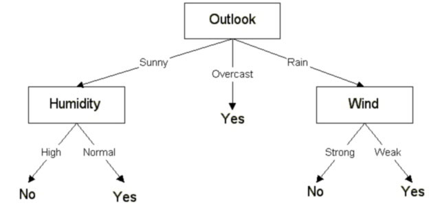
So, we'll choose the Humidity attribute for this node.
And repeat these steps, and you'll get a decision tree as below:

C4.5 Algorithm

C4.5 builds decision trees from a set of training data in the same way as ID3, using an extension to information gain known as a gain ratio.

Improvements from the ID3 algorithm

• Handling both continuous and discrete attributes;
• Handling training data with missing attribute values - C4.5 allows attribute values to be marked as ? for missing;
• Pruning trees after creation

CART Algorithm

The CART(Classification & Regression Trees) algorithm is a binary decision tree algorithm. It recursively partitions data into 2 subsets so that cases within each subset are more homogeneous. Allows consideration of misclassification costs, prior distributions, and cost-complexity pruning.

Let's take the following data as an example:

TID	Buy House	Marital Status	Taxable Income	Cheat
1	Yes	Single	125K	No
2	No	Married	100K	No
3	No	Single	70K	No
4	Yes	Married	120K	No
5	No	Divorced	95K	Yes
6	No	Married	60K	No
7	Yes	Divorced	220K	No
8	No	Single	85K	Yes
9	No	Married	75K	No
10	No	Single	90K	Yes

Firstly, we calculate the Gini Index for Buy House.

	House=Yes	House=No
Cheat=Yes	0	4
Cheat=No	3	3

So the Gini Index for this attribute should be:

• $Gini(House=Yes)=1-(\frac{3}{3})^2-(\frac{0}{3})^2=0$
• $Gini(House=Yes)=1-(\frac{4}{7})^2-(\frac{3}{7})^2=\frac{24}{49}$
• $Gini(House)=\frac{3}{10}\times{0}+\frac{7}{10}\times\frac{24}{49}=\frac{12}{35}$

How to deal with attributes with more than two values?

We calculate the Gini Index for the following splits:

• $Gini(Martial Status=Single/Divorced)$ and $Gini(Martial Status=Married)$
• $Gini(Martial Status=Single/Married)$ and $Gini(Martial Status=Divorced)$
• $Gini(Martial Status=Divorced/Married)$ and $Gini(Martial Status=Single)$

Then choose the split with a minimum Gini index.

How to deal with continuous attributes?

For efficient computation: for each attribute,

• Sort the attribute on values
• Linearly scan these values, each time updating the count matrix and computing the Gini index
• Choose the split position that has the least Gini index

Cheat	No			No		No		Yes		Yes		Yes		No		No		No		No
	Tax Income
Sorted	60			70		75		85		90		95		100		120		125		220
Split	55		65		72		80		87		92		97		110		122		172		230
	<=	>	<=	>	<=	>	<=	>	<=	>	<=	>	<=	>	<=	>	<=	>	<=	>	<=	>
Yes	0	3	0	3	0	3	0	3	1	2	2	1	3	0	3	0	3	0	3	0	3	0
No	0	7	1	6	2	5	3	4	3	4	3	4	3	4	4	3	5	2	6	1	7	0
Gini	0.420		0.400		0.375		0.343		0.417		0.400		0.300		0.343		0.375		0.400		0.420

So the value(Tax Income = 95) with minimum Gini index will be chosen as a split node.

The values will be split into two nodes: Tax Income > 97 and Tax Income <= 97.

Notes on Overfitting

Overfitting results in decision trees that are more complex than necessary. Training error no longer provides a good estimate of how well the tree will perform on previously unseen records.

Estimating Generalization Errors

Need new ways for estimating errors.

• Re‐substitution errors: error on training (Σe(t))
• Generalization errors: error on testing (Σe’(t))

Optimistic approach

Generalization errors: error on testing: e’(t) = (e(t)

Pessimistic approach

For each leaf node: e’(t) = (e(t)+0.5)

Total errors: e’(T) = e(T) + N × 0.5 (N: number of leaf nodes)

For a tree with 30 leaf nodes and 10 errors on training (out of 1000 instances):

• Training error = 10 / 1000 = 1%

Generalization error = (10 + 30 × 0.5) / 1000 = 2.5%

How to Address Overfitting

Pre‐Pruning (Early Stopping Rule)

• Stop the algorithm before it becomes a fully‐grown tree
• Typical stopping conditions for a node
  • Stop if all instances belong to the same class
  • Stop if all the attribute values are the same
• More restrictive conditions
  • Stop if the number of instances is less than some user‐specified threshold
  • Stop if the class distribution of instances is independent of the available features (e.g., using χ2 test)
  • Stop if expanding the current node does not improve impurity measures (e.g., Gini or information gain)

Post‐pruning

• Grow the decision tree to its entirety
• Trim the nodes of the decision tree in a bottom‐up fashion
• If generalization error improves after trimming, replace the sub‐tree by a leaf node
  • The class label of a leaf node is determined from the majority class of instances in the sub‐tree

Reference

• https://drive.google.com/open?id=0B4DvJHU7zJrcSk01eloxZXNkOW8
• https://en.wikipedia.org/wiki/Decision_tree
• https://en.wikipedia.org/wiki/Decision_tree_learning